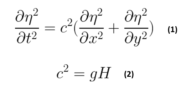
Numerical Approximation of the 2D Shallow Water Equation (constant depth)

Details:
– 2nd Order (Explicit) approximation – central in time and space
– Forcing of Shallow Water Equation with damped oscillation at center of grid
– Implementation of Boundary Conditions (Neumann & Dirichlet Boundary Conditions) and Initial Conditions
– Coded through MATLAB
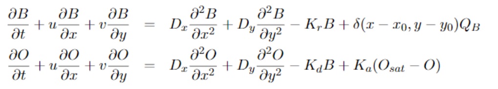
Numerical Approximation of the 2D exteneded Strecter-Phelps Equations

Details:
– Numerical approximation, first order in time and second order in space
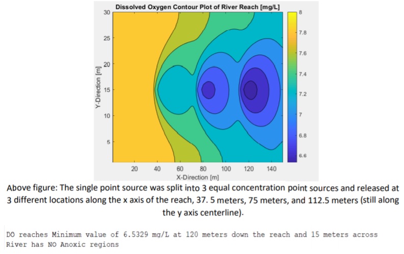
– Numerical solution of the PDE allows prediction of DO levels, when simulating the dumping of the pollutant (BOD)
-Von Neumann Stability Analysis: Peclet Number (Pe) must be 0 ≤ Pe ≤ 2
-Code displays ‘warning’ if anoxic conditions are reached (below 6 mg/L of DO)
-Allows engineers, scientist, and regulators the ability to optimize the disposal of waste (BOD), to avoid anoxic conditions (avoid violations/fines)
Stokes Drift with Turbulence
– Modeling of sediment transport, under the influence of waves & turbulence
– Three varying cases of turbulence investigated
Parameters
Wave period, T = 12 sec
Wave amplitude, a = 1 m
Water column depth, H = 10 m


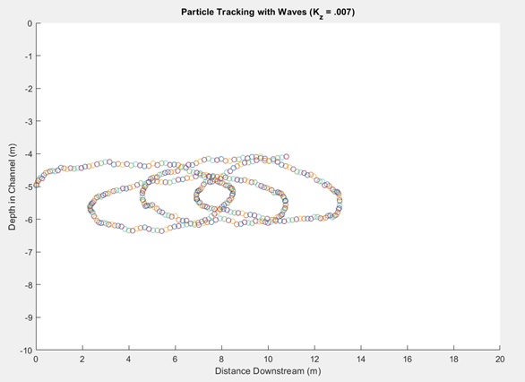

Above: Random nature of turbulence leads to a non-uniform dispersion of particles; particles forced upward due to turbulence will travel further downstream, while those forced downward will travel shorter distance
Details:
– Use of the Reynolds Average Navier- Stokes Equation (BGO/Mellor-Yamada 2-equation closure) to solve for velocity profile with incorporation of turbulence
-Increased turbulence leads to an increases in the variability of particle travel distance
-Model could be expanded to investigate other physical phenomena: influence of vegetation (increased roughness – shear stress), effect of salinity gradient (fresh and salt water interaction), and temperature gradient
